Solve an advection equation in Ruby with spitzy

A couple of days ago I started working on a collection of numerical methods for differential equations, wirtten in pure Ruby (I have conviced the professor of my numerical DE class that that`s a good idea for my final project in said class).

The Ruby gem is called spitzy. Spitzy also is this cute pomeranian. Spitzy reads backwards as yztips, which translates into:

Your Zappy-Tappy Initial value Partial (and ordinary) differential equation Solver

I set up the basic structure of the library, and implemented four methods for the 1D linear advection equation (as a start, in order to see what`s a good way to do things). The project repository is https://github.com/agisga/spitzy.git.

Below is an example of how to use spitzy in order to solve a 1D linear advection equation.

Advection Equation Example

We want to solve the 1D linear advection equation given as:

• PDE: \(\frac{du}{dt} + a \frac{du}{dx} = 0\),
• on the domain: \(0 < x < 1\) and \(0 < t < 10\),
• with periodic boundary consitions: \(u(0,t) = u(1, t)\),
• with initial condition: \(u(x,0) = \cos(2\pi x) + \frac{1}{5}\cos(10\pi x)\).

We define and solve this equation using the Upwind scheme with time steps \(dt = 0.95/1001\) and spatial steps \(dx = 1/1001\) (i.e. on a grid of 1000 equally sized intervals in \(x\)). AdvectionEq.new lets the user specify the parameters such as length of the space and time steps, time and space domain, the initial condition, etc.

require 'spitzy'
ic = proc { |x| Math::cos(2*Math::PI*x) + 0.2*Math::cos(10*Math::PI*x) }
numsol = AdvectionEq.new(xrange: [0.0,1.0], trange: [0.0, 10.0], 
                         dx: 1.0/1001, dt: 0.95/1001, a: 1.0,
                         method: :upwind, &ic)

We can get the equation solved by numsol in form of a character string using the method #equation.

There are four different numerical schemes available to solve the advection equation. Those are the Upwind, Leapfrog, Lax-Wendroff and Lax-Friedrichs methods. We can get which scheme was used by numsol with the attribute reader #method. Similarly we can access the number of \(x\)-steps #mx and \(t\)-steps #mt, as well as various other attributes.

Using Fourier methods we compute the exact solution of the PDE to be \(\cos(2\pi (x-t)) + 0.2\cos(10\pi (x-t))\). We can use it to check the accuracy of the numerical solution.

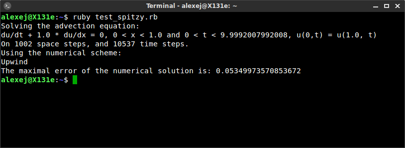
Combined, the Ruby code produces the following output (the entire code is given at the end of this post).

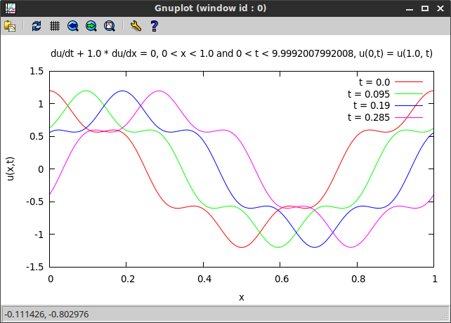
Finally, we plot the computed numerical solution at different times using the gnuplot gem (the Ruby code is given below). We use the character string numsol.equation as a header for the plot. We can see a travelling wave as expected.

require 'spitzy'

ic = proc { |x| Math::cos(2*Math::PI*x) + 0.2*Math::cos(10*Math::PI*x) }

numsol = AdvectionEq.new(xrange: [0.0,1.0], trange: [0.0, 10.0], 
                         dx: 1.0/1001, dt: 0.95/1001, a: 1.0,
                         method: :upwind, &ic)

# print the PDE to screen
puts "Solving the advection equation:"
puts numsol.equation
puts "On #{numsol.mx} space steps, and #{numsol.mt} time steps."
puts "Using the numerical scheme:"
case numsol.method
  when :upwind then puts "Upwind"
  when :leapfrog then puts "Leapfrog"
  when :lax_wendroff then puts "Lax-Wendroff"
  when :lax_friedrichs then puts "Lax-Friedrichs"
end

# compute the maximal error of the numerical solution
exactsol = proc { |x,t| Math::cos(2*Math::PI*(x-t)) + 0.2*Math::cos(10*Math::PI*(x-t)) }
u_exact = []
numsol.t.each { |t| u_exact << (0...numsol.mx).each.map { |i| exactsol.call(numsol.x[i],t) } }
u_exact.flatten!
error = []
u_num = numsol.u.flatten
(0...(numsol.mx*numsol.mt)).each { |i| error << (u_num[i] - u_exact[i]).abs }
maxerror = error.max
puts "The maximal error of the numerical solution is: #{maxerror}\n"

# plot the numerical solution
require 'gnuplot'
def plot(title, numsol, *t_indices)
  Gnuplot.open do |gp|
    Gnuplot::Plot.new(gp) do |plot|
      plot.title title.to_s
      plot.xlabel "x"
      plot.ylabel "u(x,t)"

      t_indices.each do |i|
        x = numsol.x
        y = numsol.u[i]
        plot.data << Gnuplot::DataSet.new([x,y]) do |ds|
          ds.with = "lines"
          ds.title = "t = #{numsol.t[i].round(3)}"
        end
      end
    end
  end
end

plot(numsol.equation, numsol, 
     0, 10, 20, 40)