A rudimentary first linear mixed model fit
During the last two weeks I made some progress on my Google Summer of Code project.
The Ruby gem is now capable of fitting linear mixed models. In this short blog post I want to give an example, and compare the results I get in Ruby to those obtained by lme4 in R.
LMM Mathematical Basics
Mathematically, a linear mixed model has the general form
\[(y | b = \hat{b}) \sim \mathrm{N}(X\beta + Z\hat{b} + o, \sigma^2 W^{-1}), \mathrm{\,with\,} b \sim \mathrm{N}(0, \Sigma\subscript{\theta}),\]where \(y\in\mathbb{R}^n\) and \(b\in\mathbb{R}^q\) are random vectors (response and random effects), \(\beta\in\mathbb{R}^p\) is the vector of fixed effects, \(o\in\mathbb{R}^n\) is a vector of known prior offset terms, \(W\in\mathbb{R}^{n\times n}\) is a diagonal matrix of known prior weights. The random effects covariance matrix \(\Sigma\subscript{\theta}\in\mathbb{R}^{q\times q}\) depends on the variance component parameter vector \(\theta\in\mathbb{R}^l\). Additionally, via the Cholesky decomposition we write
\[\Sigma\subscript{\theta} = \sigma^2 \Lambda\subscript{\theta} \Lambda\subscript{\theta}^T,\]where \(\Lambda\subscript{\theta}\) is a lower triangular matrix, which is parametrized by \(\theta\) in a way that is known a priori.
The goal of the model fitting process is to find parameter estimates \(\hat{\theta}\), \(\hat{\beta}\) and \(\hat{b}\) that fit the observed data best. Then the LMM fit can be used for prediction and inference.
Model Fit Example
The only currently available user interface is rudimentary. It requires the user to set up the design matrix \(X\), the random effects model matrix \(Z\), a Proc that generates a \(\Lambda\subscript{\theta}\) matrix from a \(\theta\) input, etc. by hand, before calling LMM#initialize. On the bright side, this adds a lot of flexibility to the model specification. In the future, I will write a more user-friendly R-like method LMM#from_formula.
The Data
Now, let’s look at the simulated data that I use to test the implemented method.
I generate a 50x2 design matrix \(X\) with one column of ones (for the intercept) and one column of numbers 1,2,3,…,50. The data is divided into five groups of equal size (consecutive blocks of 10 rows of \(X\)). Each of these groups has its own random intercept and random slope. Thus, the random effects model matrix \(Z\) is of size 50x10, and has the form
1 1  0 0  0 ...
1 2  0 0  0 ...
   ....
1 10 0 0  0 ...
0 0  1 11 0 ...
0 0  1 12 0 ...
   ....
0 0  1 20 0 ...
   ....
and \(\Lambda\subscript{\theta}\) is 10x10 block-diagonal with five square blocks of the form [ [theta[0], 0], [theta[1], theta[2] ].
The random effects b are generated from the multivariate distribution with mean 0 and covariance matrix [ [1, 0.5], [0.5, 1] ], and 50 random error terms epsilon are generated from the standard normal distribution. Both, the fixed intercept and slope are set to be equal to one.
Finally I generate the response vector y as
y = (x.dot beta) + (z.dot b) + epsilon
Results
The model fit can be performed with MixedModels in Ruby via:
model_fit = LMM.new(x: x, y: y, zt: z.transpose, lambdat: lambdat,
start_point: [1,0,1], lower_bound: Array[0,-Float::INFINITY,0],
¶metrization)
My entire Ruby code for this example can be found on github here.
Behind the scenes, LMM#initialize essentially performs the following three steps:
# (1) Create the data structure in a LMMData object
@model_data = LMMData.new(x: x, y: y, zt: zt, lambdat: lambdat,
                          weights: weights, offset: offset, &thfun)

# (2) Set up the profiled deviance/REML function
@dev_fun = MixedModels::mk_lmm_dev_fun(@model_data, @reml)

# (3) Optimize the deviance/REML
@optimization_result = MixedModels::NelderMead.minimize(start_point: start_point,
                                                        lower_bound: lower_bound,
                                                        upper_bound: upper_bound,
                                                        epsilon: epsilon,
                                                        max_iterations: max_iterations,
                                                        &dev_fun)
We can fit a linear mixed model in R to the same matrix and vector data with:
dat.frm <- as.data.frame(cbind(y, X[,2], rep(1:5,each=10)))
names(dat.frm) <- c("y", "x", "grp")
lmer.fit <- lmer(y~x+(x|grp), dat.frm)
Let’s look at some of the results.
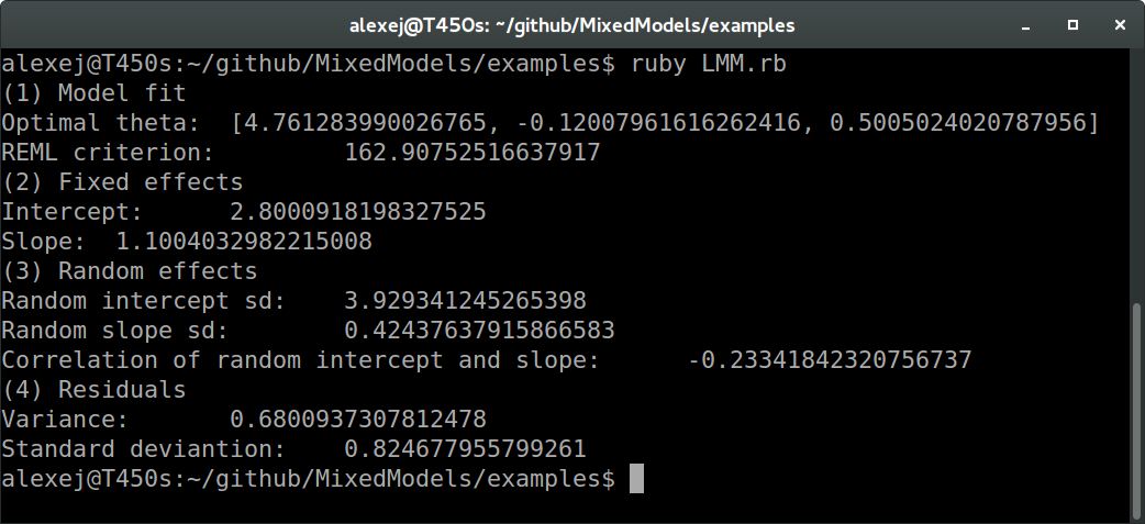
In Ruby:

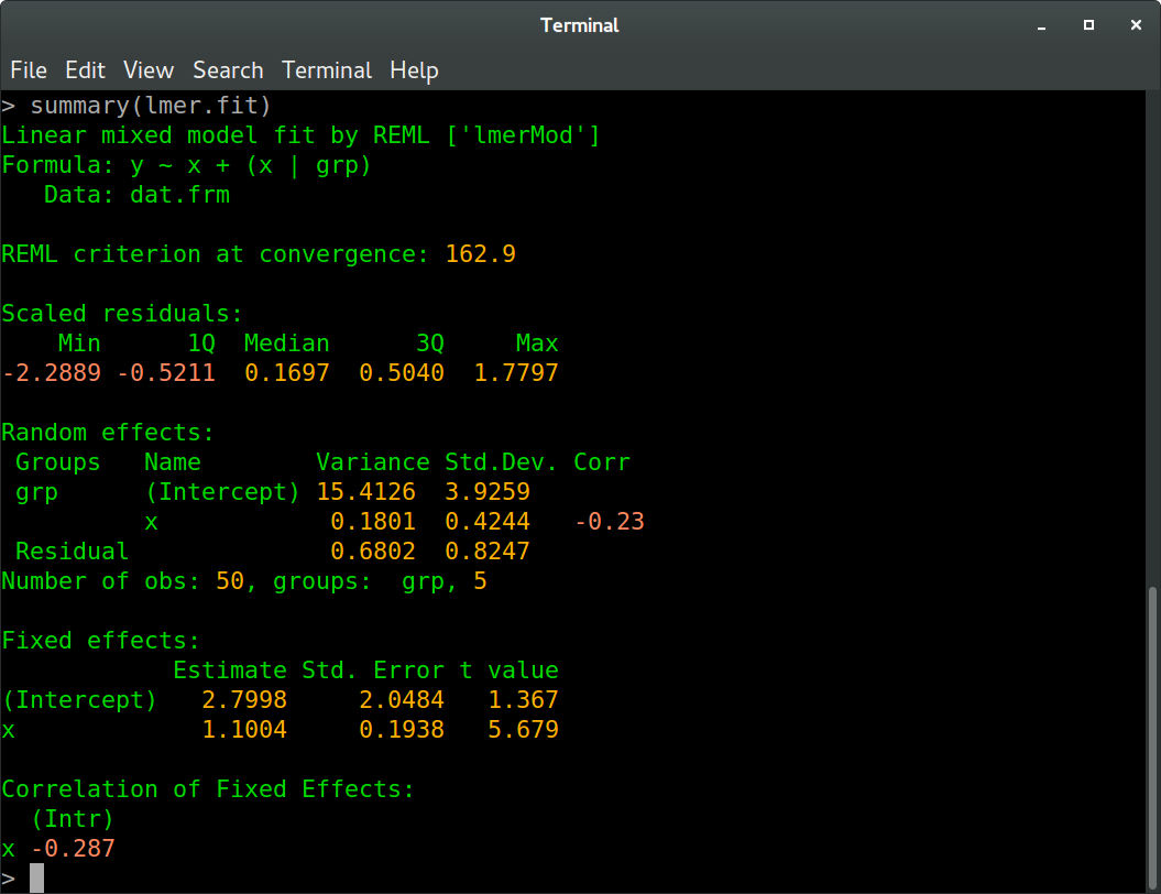
And in R:

We see that all values agree between Ruby and R up to at least one digit behind the floating point (these values are the REML criterion, fixed effects estimates, random effects standard deviations and correlation, and residual variance and standard deviation, to be more precise). The slight differences are probably due to different optimization routines.