Dissecting lme4's lmer function. Part 2.
Last time I started to analyze the function lmer that is used to fit linear mixed models in the R package lme4. I have delineated the general steps taken by lmer, and looked at the employed formula module in more detail. The formula module evaluates the provided R model formula to model matrices, vectors and parameters. The next step is to use these to define the objective function that needs to be minimized, which is the profiled deviance or the profiled REML criterion in this case. The objective function is returned by the function mkLmerDevfun which is dissected in what follows.
Set up the deviance function - “mkLmerDevfun”
Much of the code of mkLmerDevfun and the functions called from therein deals with the situation when the user wants to fit a generalized or nonlinear mixed model, but calls lmer instead of other respectively designated functions. Then the code repackages the provided function arguments and passes them to the respective function (which should have been called by the user in the first place). I will disregard such passages of the code, because I’m only interested in the linear mixed model capabilities right now (besides, I find that it would have been a better design to simply abort the function execution with a warning in such cases).
Okay, now let’s dislimb, dismember and dissect!
The function mkLmerDevfun is defined in the file modular.R as:
mkLmerDevfun <- function(fr, X, reTrms, REML = TRUE, start = NULL, verbose=0, control=lmerControl(), ...)
It begins by extracting some variables from the function call, most importantly:
rho- a new environment with the parent being the environment from whichmkLmerDevfunwas called (containing who knows what…),rho$pp- a newmerPredDobject, which stores the dense model matrixX, the transpose of the sparse model matrix for the random effectsZt,Lambdatthe transpose of the sparse lower triangular relative variance,Lindinteger vector of the same length as thexslot in theLambdatfield (I don’t know yet what it’s for),thetanumeric vector of variance component parameters,nsample size, and other auxiliary parameters computed from these.rho$resp- anlmerRespobject, which essentially holds the response vector \(y\), and additionally some associated parameters (like the weights for each observation, offset terms and others), as well as the REML flag.
Then mkLmerDevfun diverts to the function mkdevfun (defined in lmer.R), which takes as input the environment rho and returns a function devfun with rho as an associated environment. The function mkdevfun sets
rho$lmer_Deviance <- lmer_Deviance
and defines devfun as
function(theta) .Call(lmer_Deviance, pp$ptr(), resp$ptr(), as.double(theta))
I inspect the C++ function lmer_Deviance in great detail below.
If all random effects are intercept terms (i.e. the covariance matrix of \(y\) is diagonal with entries \(\theta\subscript{i}\)) and no starting values are provided, the function mkLmerDevfun continues by computing starting values for \(\theta\) as \(\sqrt{v / v\subscript{e}}\), where \(v\) is a vector with as many entries as there are random terms, containing in each entry the sample variance of \((\bar{y}\subscript{\cdot 1},\ldots,\bar{y}\subscript{\cdot 1}, \bar{y}\subscript{\cdot 2},\ldots,\bar{y}\subscript{\cdot 2}, \ldots)^T\), and \(v\subscript{e} = \mathrm{Var}(y) - \sum v\subscript{i}\) (in usual notation \(\bar{y}\subscript{\cdot 1}\) denotes the average of the sample values in \(y\) belonging to the first level of the random effect). That is, in more intuitive terms the starting value for \(\theta\subscript{i}\) is the standard deviation due to the \(i\)th random effect scaled by the residual standard deviation.
If not all random effects are intercept terms, then the initial values for \(\theta\) are 0 off-diagonal and 1 on, as defined via the function mkReTrms called from the function lFormula prior to the call of mkLmerDevfun.
Finally, devfun is returned, which should also pass the rho environment implicitly.
lmer_Deviance
This function is defined as SEXP lmer_Deviance(SEXP pptr_, SEXP rptr_, SEXP theta_) in external.cpp.
Using the Rcpp:::Xptr template, it creates two external pointers to instances of the C++ classes lmerResp and merPredD, thus exposing all methods of the respective C++ objects to the use from R.
XPtr<lmerResp>   rpt(rptr_);
XPtr<merPredD>   ppt(pptr_);
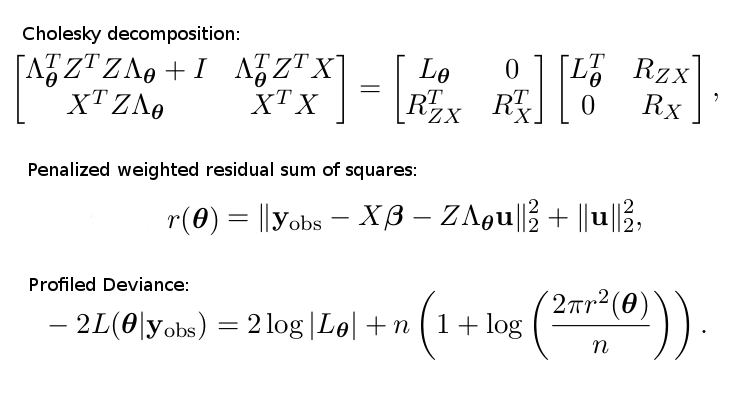
The function proceeds by calling another function, lmer_dev, defined in the same file, which carries out the actual computation of the (profiled) deviance function. The mathematical expression of the profiled deviance is essentially given by the following set of formulas (as I have derived in my project plan here: http://dauns.math.tulane.edu/~agossman/pdfs/GSoC2015_LMM_project_plan.pdf).

The Cholesky decomposed matrix is part of a linear system, predicting the random terms \(u\) and the coefficient vector \(\beta\).
These math formulas are evaluated in lmer_dev via the following steps:
-
ppt->setTheta(theta)- Update the parameter vector \(\theta\) and the covariance factor \(\Lambda\subscript{\theta}\). -
ppt->updateXwts(rpt->sqrtXwt())- Update the matrix \(W\) of \(X\) weights. \(W\) is not shown above for simplicity, but in fact there is a factor \(W^{1/2}\) in front of every \(X\) or \(Z\) in the above formulas. -
rpt->updateMu(ppt->linPred(0.))- Update the (conditional) mean response, the weighted residuals vector, and its sum of squares, based ond_beta0andd_u0. -
ppt->updateRes(rpt->wtres())- Does these auxiliary calculations:
d_Vtr = d_V.adjoint() * wtres;
d_Utr = d_LamtUt * wtres;
(I don’t really understand the purpose of it at the moment).
-
ppt->solve()- Performs the above Cholesky decomposition in multiple steps viaCHOLMODsparse Cholesky methods (possibly also estimates \(u\) and maybe some other parameters, but I am not sure). -
rpt->updateMu(ppt->linPred(1.))- Update the (conditional) mean response, the weighted residuals vector, and its sum of squares, based ond_beta0 + d_delbandd_u0 + d_delu. -
val=rpt->Laplace(ppt->ldL2(), ppt->ldRX2(), ppt->sqrL(1.))- Evaluate the profiled deviance based on the previously computed variables (or the profiled REML criterion, which is defined similarly, if the REML flag is set). -
Return
val.
It seems that the implementation in the package lme4pureR performs all the same calculations, but is written in a much better readable R code (much fewer lines of code, without external pointers to C++ objects and no C++/C used at all, without passing different R environments from function to function, etc.). I will look at it in detail as soon as I finish dissecting lme4’s lmer.