Concordance Correlation Coefficient
If we collect \(n\) independent pairs of observations \((y_{11}, y_{12}), (y_{21}, y_{22}), \dots, (y_{n1}, y_{n2})\) from some bivariate distribution, then how can we estimate the expected squared perpendicular distance of each such point in the 2D plane from the 45-degree line?
Assume that the random two-dimensional vector \((Y_1, Y_2)\) follows a bivariate distribution with mean \(\E(Y_1, Y_2) = (\mu_1, \mu_2)\), and covariance matrix with entries \(\mathrm{Var}(Y_1) = \sigma_1^2\), \(\mathrm{Var}(Y_2) = \sigma_2^2\) and \(\mathrm{Cov}(Y_1, Y_2) = \sigma_{12}\).
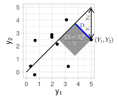
The squared perpendicular distance of the random point \((Y_1, Y_2)\) from the 45-degree line is
\[\begin{equation*} D^2 = \frac{(Y_1 - Y_2)^2}{2}, \end{equation*}\]see the figure below. Thus, the expected value of the squared perpendicular distance times two (for notational convenience) is given by,
\[\begin{align} \E\left[ 2D^2 \right] &= \E\left[ (Y_1 - Y_2)^2 \right] \nonumber \\ &= \E\left[ \left( (Y_1-\mu_1) - (Y_2-\mu_2) + \mu_1-\mu_2 \right)^2 \right] \nonumber \\ &= \E\left[ \left((Y_1-\mu_1) - (Y_2-\mu_2) \right)^2 \right] + (\mu_1-\mu_2)^2 \nonumber \\ &= (\mu_1-\mu_2)^2 + \sigma_1^2 + \sigma_2^2 - 2\sigma_{12} \label{eq:decomp1} \\ &= (\mu_1-\mu_2)^2 + (\sigma_1 - \sigma_2)^2 + 2[1 - \rho] \sigma_1 \sigma_2. \nonumber \end{align}\]To answer the question raised above, we can estimate the value of equation \(\eqref{eq:decomp1}\) based on \(n\) pairs of observations \((y_{11}, y_{12}), (y_{21}, y_{22}), \dots, (y_{n1}, y_{n2})\) substituting the respective sample mean, sample variance, and covariance estimates for \(\mu_1, \mu_2, \sigma_1^2, \sigma_2^2, \sigma_{12}\) respectively.
Defining the Concordance Correlation Coefficient
That’s great, but why should we spend any time thinking about the expected distance from the 45-degree line? What’s interesting about it?
Apart from delighting in the pure joy of doing mathematics and taking pleasure in the experience of mathematical beauty… ![]()
![]() …
A measure of distance from the 45-degree line naturally quantifies the (dis)agreement between the two sets of observations.
For example, we may have measured the same target entities using two different measurement instruments, and may want to know if and to what extent they agree.
…
A measure of distance from the 45-degree line naturally quantifies the (dis)agreement between the two sets of observations.
For example, we may have measured the same target entities using two different measurement instruments, and may want to know if and to what extent they agree.
Towards quantifying the extent of the (dis)agreement between two sets of observations it is natural to try to scale (or normalize) the quantity of equation \(\eqref{eq:decomp1}\) to the range \([0, 1]\). However, it turns out that, rather than scaling to a \([0, 1]\) range, it is customary to scale this quantity to the range from -1 to 1 as follows,
\[\begin{equation} \mathrm{CCC} := 1 - \frac{\E\left[ (Y_1 - Y_2)^2 \right]}{(\mu_1-\mu_2)^2 + \sigma_1^2 + \sigma_2^2} = \frac{2\sigma_{12}}{(\mu_1-\mu_2)^2 + \sigma_1^2 + \sigma_2^2}. \label{eq:ccc} \end{equation}\]This expression, first introduced by (Lin, 1989), is known as the Concordance Correlation Coefficient, abbreviated as CCC hereafter.
Concordance Correlation Coefficient vs. Pearson correlation coefficient
The scaling into the range from -1 to 1 may have been motivated by the fact that the Pearson correlation coefficient \(\rho\) also falls within the \([-1, 1]\) range. In fact, analogous to how a Pearson correlation coefficient \(\rho=1\) signifies perfect positive correlation, a CCC of 1 designates that the paired observations fall exactly on the line of perfect concordance (i.e., the 45-degree diagonal line).
Further aspects of the relationship to the Pearson correlation coefficient \(\rho\) become visible if we rewrite the CCC further into the following set of equations.
\[\begin{equation} \mathrm{CCC} = \rho C, \label{eq:ccc2} \end{equation}\]where
\[\begin{equation} C = \frac{2}{v + \frac{1}{v} + u^2}, v = \frac{\sigma_1}{\sigma_2}, u = \frac{(\mu_1 - \mu_2)^2}{\sigma_1 \sigma_2}. \label{eq:c} \end{equation}\]From equations \(\eqref{eq:ccc2}\) and \(\eqref{eq:c}\) we observe that:
- CCC always has the same sign as \(\rho\).
- CCC is 0 if and only if \(\rho = 0\) (with exception of cases when \(\rho\) is undefined but CCC can still be computed via equation \(\eqref{eq:ccc}\)).
- We can consider \(\rho\) to be a measure of precision, i.e., how far each point deviates from the best fitting line. Thus, CCC combines \(\rho\) (as a measure of precision) with an additional measure of accuracy denoted by \(C\) in equations \(\eqref{eq:ccc2}\) and \(\eqref{eq:c}\), whereby:
- \(C\) quantifies how far the best-fit line deviates from the 45-degree line.
- When the data lie exactly on the 45-degree line, then we have that C = 1. The further the observations deviate from the 45-degree line, the further C is from 1 and the closer it is to 0.
- In particular, \(v\) from equation \(\eqref{eq:c}\) can be considered a measure of scale shift, and \(u\) from equation \(\eqref{eq:c}\) a measure of location shift relative to the scale.
Now it turns out that the Pearson correlation coefficient \(\rho\) has one major shortcoming when assessing reproducibility of measurements, such as when comparing two instruments that measure the same target entity.
![]() Unlike CCC, \(\rho\) is invariant to additive or multiplicative shifts by a constant value, referred to as location shift and scale shift respectively in the following set of figures:
Unlike CCC, \(\rho\) is invariant to additive or multiplicative shifts by a constant value, referred to as location shift and scale shift respectively in the following set of figures:
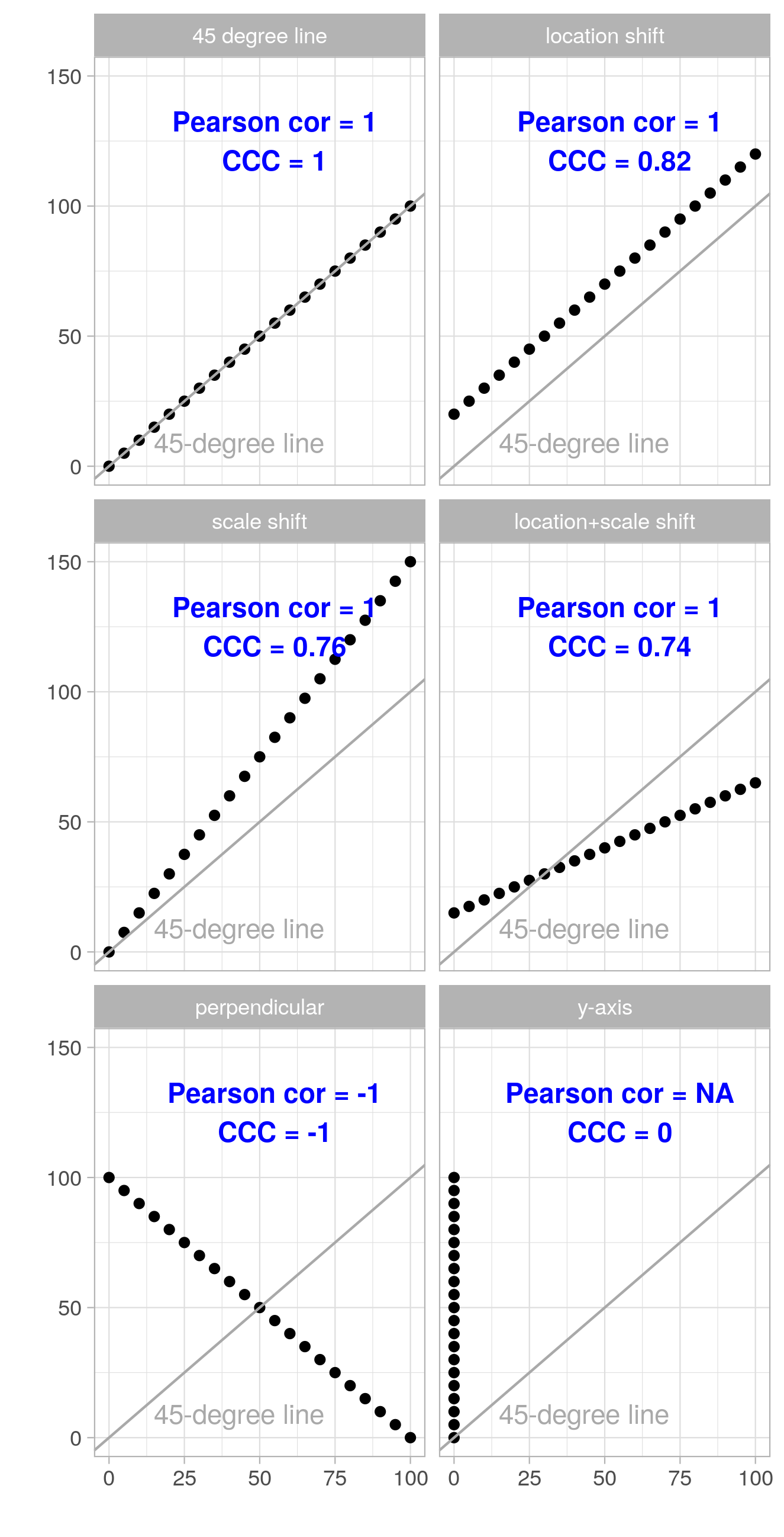
Looking at the above figures we see that the magnitude of the Pearson correlation coefficient \(\rho\) does not change under location and scale shift (though the sign may flip). The CCC on the other hand quantifies the deviation from the 45-degree line, which is due to location and scale shifts in these examples, rather well.
This makes the CCC a better metric when we want to assess how well one measurement can reproduce another (i.e., how close the measurement pairs fall to the 45-degree line), while we would use \(\rho\) if what we want is quantifying to what extent the measurement pairs can be described by a linear equation (with any intercept and slope).
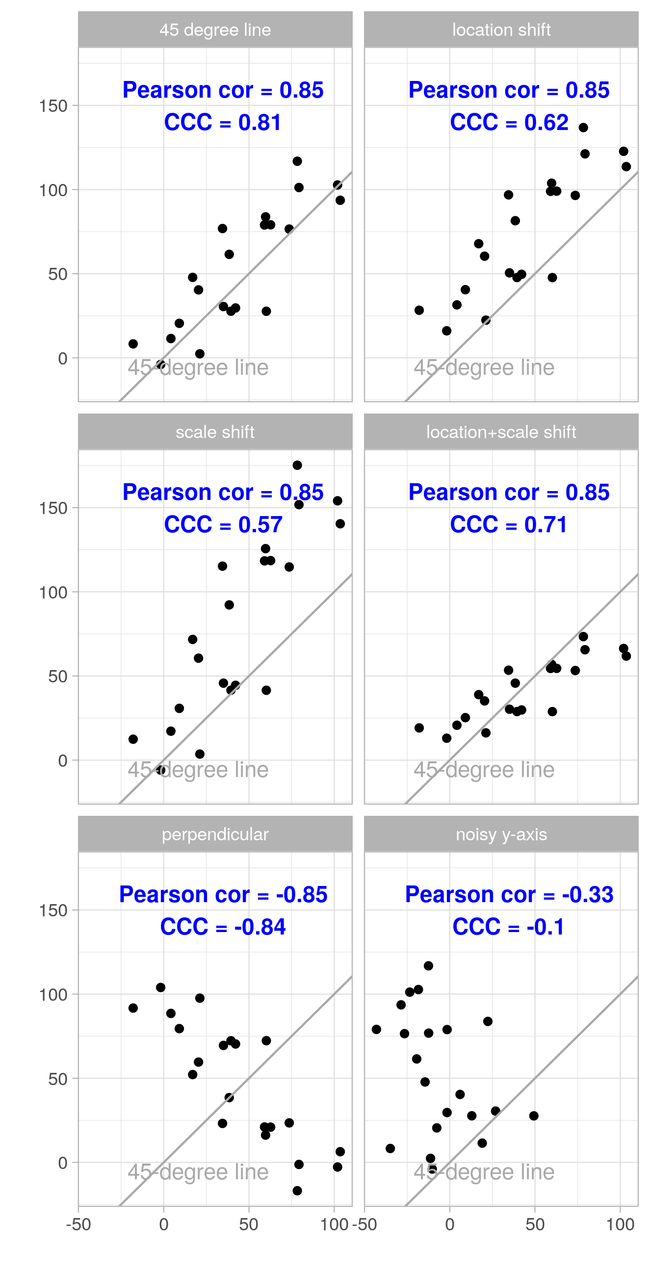
The following figures show the same examples where both the \(x\) and the \(y\) coordinates are augmented with Gaussian noise (mean 0, standard deviation 15; the same realization of the random noise is used within each subfigure). We see that both \(\rho\) and CCC move further away from the extreme values of \(-1\), \(0\), and \(1\) as noise is added.
What’s CCC good for? Reproducibility?
As hinted above, you may want to compare two instruments that aim to measure the same target entity, or two assays that aim to measure the same analyte, or other quantitative measurement procedures or devices. For example, one set of measurements may be obtained by what’s considered the “gold standard”, while the other set of measurements may be collected by a new instrument/assay/device that may be cheaper or in some other way preferable to the “gold standard” instrument/assay/device. Then one would wish to demonstrate that the collected two sets of measurements are equivalent. (Lin, 1989) refers to this type of agreement or similarity between two sets of measurements as reproducibility of measurements. The paper considers the following two illustrative examples:
(1) Can a “Portable $ave” machine (actual name withheld) reproduce a gold-standard machine in measuring total bilirubin in blood?
(2) Can an in-vitro assay for screening the toxicity of biomaterials reproduce from trial to trial?
And indeed this type of reproducibility assessment is a task where CCC has some clear advantages over the Pearson correlation coefficient, as seen in the figures above, as well as over some other approaches, as discussed in (Lin, 1989) in detail. A couple of shortcomings of common statistical approaches (when applied to the reproducibility assessment problem in question) are the following:
- The paired t-test can reject a highly reproducible set of measurements when the variance is very small, while it fails to detect poor agreement in pairs of data when the means are equal.
- The least squares approach of testing intercept equal to 0 and slope equal to 1 fails to detect nearly perfect agreement when the residual errors are very small, while it has increasingly little chance to reject the null hypothesis of agreement the more the data are scattered.
I will end here. However, if you want to go deeper into the topic I invite you to check out the original paper by Lin for a more thorough discussion of the merits of the CCC as well as for its statistical properties. Moreover, since the publication of (Lin, 1989) there of course has been follow-up work, which I didn’t read (so, I may update this blog post in the future).
References
- Lin, L. I. (1989). A concordance correlation coefficient to evaluate reproducibility. Biometrics, 45(1), 255–268. https://www.ncbi.nlm.nih.gov/pubmed/2720055