From conditional probability to conditional distribution to conditional expectation, and back

I can’t count how many times I have looked up the formal (measure theoretic) definitions of conditional probability distribution or conditional expectation (even though it’s not that hard ) Another such occasion was yesterday. This time I took some notes.

From conditional probability → to conditional distribution → to conditional expectation

Let \(X\) and \(Y\) be two real-valued random variables.

Conditional probability

For a fixed set \(B\) (Feller, 1966, p. 157) defines conditional probability of an event \(\{Y \in B\}\) for given \(X\) as follows.

By \(\prob(Y \in B \vert X)\) (in words, “a conditional probability of the event \(\{Y \in B\}\) for given \(X\)”) is meant a function \(q(X, B)\) such that for every set \(A \in \mathbb{R}\)

\[\prob(X \in A, Y \in B) = \int_A q(x, B) \mu(dx)\]

where \(\mu\) is the marginal distribution of \(X\).

(where \(A\) and \(B\) are both Borel sets on \(\R\).)

That is, the conditional probability can be defined as something that, when integrated with respect to the marginal distribution of \(X\), results in the joint probability of \(X\) and \(Y\).

Moreover, note that if \(A = \R\) then the above formula yields \(\prob(Y \in B)\), the marginal probability of the event \(\{ Y \in B \}\).

Example

For example, if the joint distribution of two random variables \(X\) and \(Y\) is the following bivariate normal distribution

\[\begin{pmatrix} X \\ Y \end{pmatrix} \sim \mathcal{N} \left( \begin{pmatrix} \mu_X \\ \mu_Y \end{pmatrix}, \begin{pmatrix} \sigma^2_X & \rho \sigma_X \sigma_Y \\ \rho \sigma_X \sigma_Y & \sigma^2_Y \end{pmatrix} \right),\]

then by sitting down with a pen and paper for some amount of time, it is not hard to verify that the function

\[q(x, B) = \int_B \frac{1}{\sqrt{2\pi(1-\rho^2)}\sigma_Y} \exp\left(-\frac{\left(y - \mu_Y+\frac{\sigma_Y}{\sigma_X}\rho( x - \mu_X)\right)^2}{2(1-\rho^2)\sigma_Y^2}\right) \mathrm{d}y\]

in this case satisfies the above definition of \(\prob(Y \in B \vert X)\).

Conditional distribution

Later on (Feller, 1966, p. 159) follows up with the notion of conditional probability distribution:

By a conditional probability distribution of \(Y\) for given \(X\) is meant a function \(q\) of two variables, a point \(x\) and a set \(B\), such that

1. for a fixed set \(B\)

   \[q(X, B) = \prob(Y \in B \vert X )\]

   is a conditional probability of the event \(\{Y \in B\}\) for given \(X\).

2. \(q\) is for each \(x\) a probability distribution.

It is also pointed out that

In effect a conditional probability distribution is a family of ordinary probability distributions and so the whole theory carries over without change.

(Feller, 1966)

When I first came across this viewpoint, I found it incredibly enlightening to regard the conditional probability distribution as a family of ordinary probability distributions.

Example

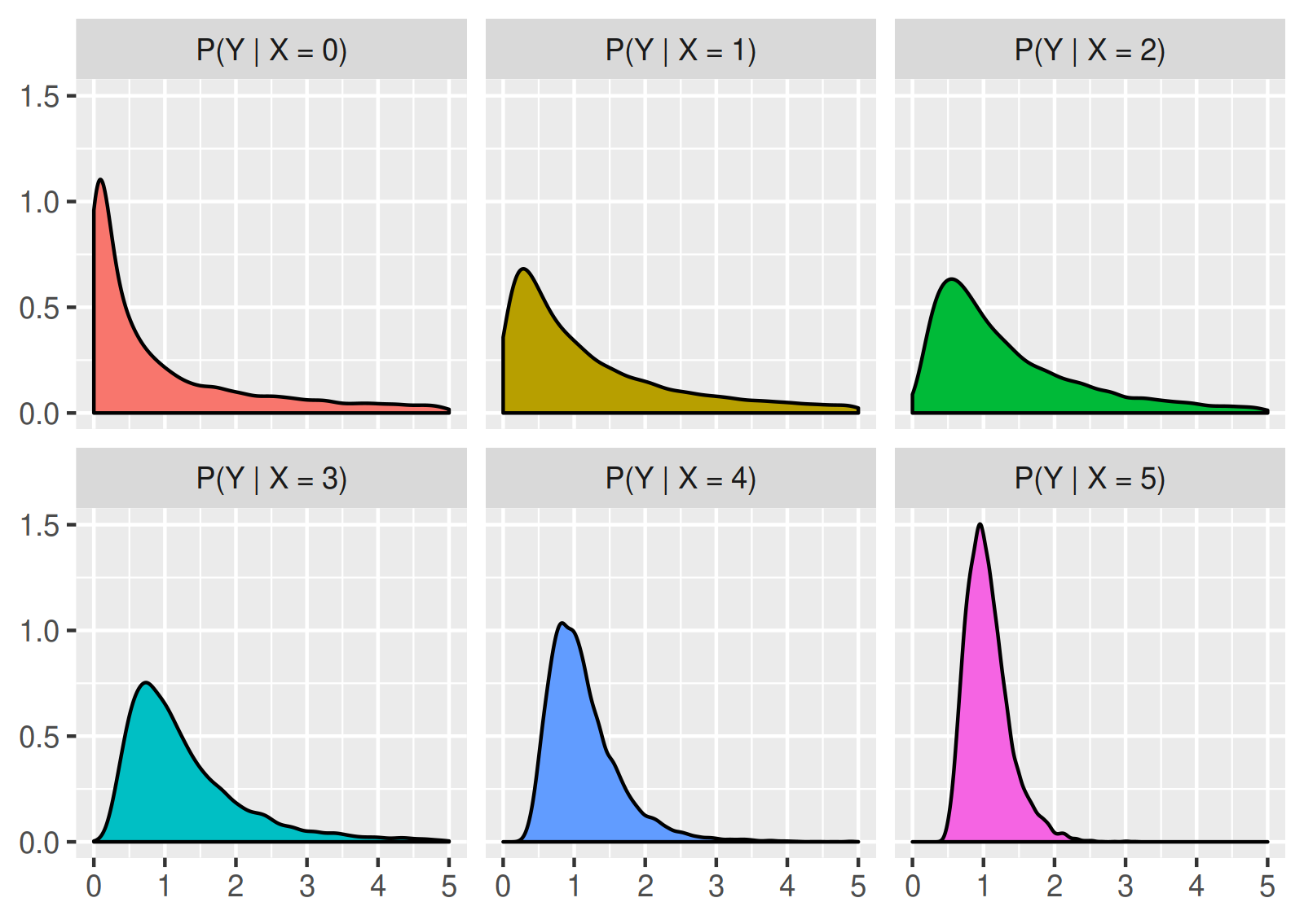
For example, assume that \(X\) is an integer-valued and non-negative random variable, and that the conditional probability distribution of \(Y\) for given \(X\) is an F-distribution (denoted \(\mathrm{F}(d_1, d_2)\)) with \(d_1 = e^X\) and \(d_2 = 2^X\) degrees of freedom. Then the conditional probability distribution of \((Y \vert X)\) can be regarded as a family of probability distributions \(\mathrm{F}(e^x, 2^x)\) for \(x = 0, 1, 2, \dots\), whose probability density functions look like this:

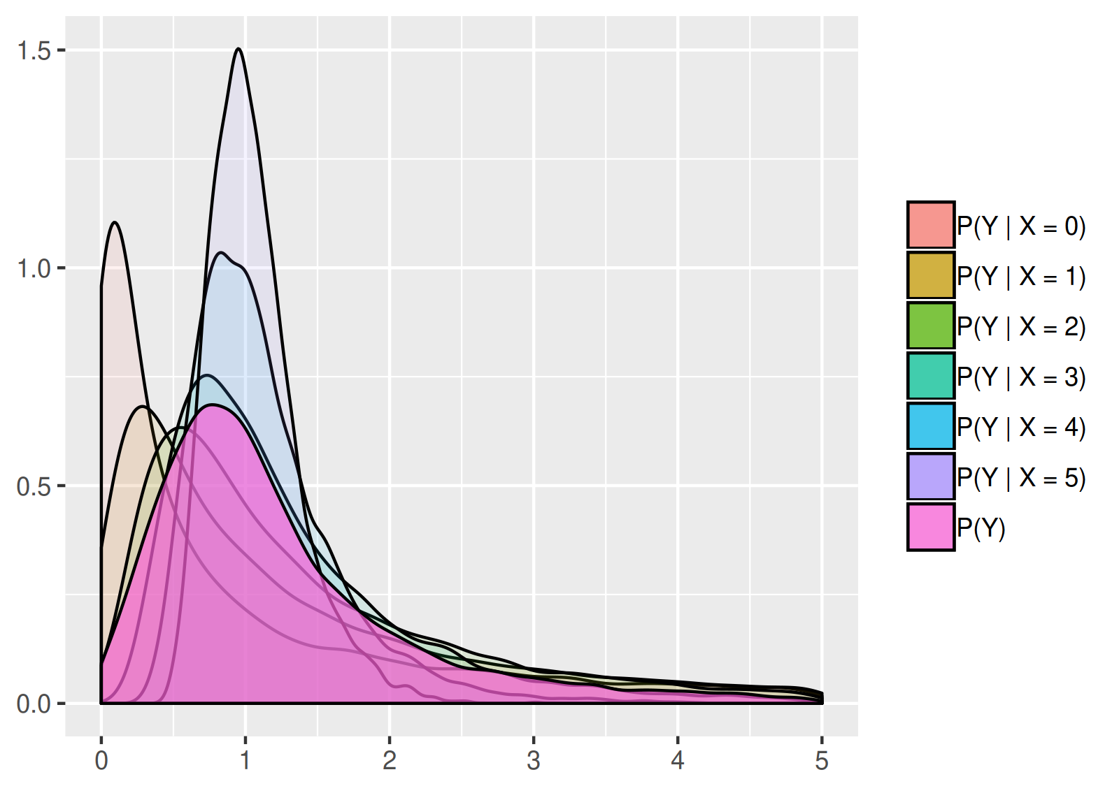
In addition, as pointed out above, if we know the marginal distribution of \(X\), then the conditional probability distribution of \((Y \vert X)\) can be used to obtain the marginal probability distribution of \(Y\), or to randomly sample from the marginal distribution. Practically it means that if we randomly generate a value of \(X\) according to its probability distribution, and use this value to randomly generate a value of \(Y\) according to the conditional distribution of \(Y\) for the given \(X\), then the observations resulting from this procedure follow the marginal distribution of \(Y\). Continuing the previous example, assume that \(X\) follows a binomial distribution with parameters \(n = 5\) and \(p = 0.5\). Then the described simulation procedure estimates the following shape for the probability density function of \(\prob(Y)\), the marginal distribution of \(Y\):

Conditional expectation

Finally, (Feller, 1966, p. 159) introduces the notion of conditional expectation. By the above, for given a value \(x\) we have that

\[q(x, B) = \prob(Y \in B \vert X = x), \quad\forall B\in\mathcal{B}\]

(here \(\mathcal{B}\) denotes the Borel \(\sigma\)-algebra on \(\R\)), and therefore, a conditional probability distribution can be viewed as a family of ordinary probability distributions (represented by \(q\) for different \(x\)s). Thus, as (Feller, 1966, p. 159) points out, if \(q\) is given then the conditional expectation “introduces a new notation rather than a new concept.”

A conditional expectation \(E(Y \vert X)\) is a function of \(X\) assuming at \(x\) the value

\[\E(Y \vert X = x) = \int_{-\infty}^{\infty} y q(x, dy)\]

provided the integral converges.

Note that, because \(\E(Y \vert X)\) is a function of \(X\), it is a random variable, whose value at an individual point \(x\) is given by the above definition. Moreover, from the above definitions of conditional probability and conditional expectation it follows that

\[\E(Y) = \E(\E(Y \vert X)).\]

Example [cont.]

We continue with the last example. From the properties of the F-distribution we know that under this example’s assumptions on the conditional distribution, it holds that

\[\E(Y \vert X = x) = \begin{cases} \frac{d_2}{d_2 - 2} = \frac{2^x}{2^x - 2}, \quad x > 1,\\ \infty, \quad x \leq 1. \end{cases}\]

A rather boring strictly decreasing function of \(x\) converging to \(1\) as \(x\to\infty\).

Thus, under the example’s assumption on the distribution of \(X\), the conditional expectation \(\E(Y \vert X)\) is a discrete random variable, which has non-zero probability mass at the values \(2, 4/3, 8/7, 16/15,\) and \(\infty\).

From conditional expectation → to conditional probability

An alternative approach is to define the conditional expectation first, and then to define conditional probability as the conditional expectation of the indicator function. This approach seems less intuitive to me. However, it is more flexible and more general, as we see below.

Conditional expectation

A definition in 2D

Let \(X\) and \(Y\) be two real-valued random variables, and let \(\mathcal{B}\) denote the Borel \(\sigma\)-algebra on \(\R\). Recall that \(X\) and \(Y\) can be represented as mappings \(X: \Omega \to \R\) and \(Y: \Omega \to \R\) over some measure space \((\Omega, \mathcal{A}, \prob)\). We can define \(\mathrm{E}(Y \vert X=x)\), the conditional expectation of \(Y\) given \(X=x\), as follows.

A \(\mathcal{B}\)-measurable function \(g(x)\) is the conditional expectation of \(Y\) for given \(x\), i.e.,

\[\mathrm{E}(Y \vert X=x) = g(x),\]

if for all sets \(B\in\mathcal{B}\) it holds that

\[\int_{X^{-1}(B)} Y(\omega) d\prob(\omega) = \int_{B} g(x) d\prob^X(x),\]

where \(\prob^X\) is the marginal probability distribution of \(X\).

Interpretation in 2D

If \(X\) and \(Y\) are real-valued one-dimensional, then the pair \((X,Y)\) can be viewed as a random vector in the plane. Each set \(\{X \in A\}\) consists of parallels to the \(y\)-axis, and we can define a \(\sigma\)-algebra induced by \(X\) as the collection of all sets \(\{X \in A\}\) on the plane, where \(A\) is a Borel set on the line. The collection of all such sets forms a \(\sigma\)-algebra \(\mathcal{A}\) on the plane, which is contained in the \(\sigma\)-algebra of all Borel sets in \(\R^2\). \(\mathcal{A}\) is called the \(\sigma\)-algebra generated by the random variable \(X\).

Then \(\mathrm{E}(Y \vert X)\) can be equivalently defined as a random variable such that

\[\mathrm{E}(Y\cdot I_{A}) = \mathrm{E}(\mathrm{E}(Y \vert X) \cdot I_{A}), \quad \forall A\in\mathcal{A},\]

where \(I_{A}\) denotes the indicator function of the set \(A\).

A more general definition of conditional expectation

The last paragraph illustrates that one could generalize the definition of the conditional expectation of \(Y\) given \(X\) to the conditional expectation of \(Y\) given an arbitrary \(\sigma\)-algebra \(\mathcal{B}\) (not necessarily the \(\sigma\)-algebra generated by \(X\)). This leads to the following general definition, which is stated in (Feller, 1966, pp. 160-161) in a slightly different notation.

Let \(Y\) be a random variable, and let \(\mathcal{B}\) be a \(\sigma\)-algebra of sets.

1. A random variable \(U\) is called a conditional expectation of \(Y\) relative to \(\mathcal{B}\), or \(U = \E(Y \vert \mathcal{B})\), if it is \(\mathcal{B}\)-measurable and

   \[\E(Y\cdot I_{B}) = \E(U \cdot I_{B}), \quad \forall B\in\mathcal{B}.\]

2. If \(\mathcal{B}\) is the \(\sigma\)-algebra generated by a random variable \(X\), then \(\E(Y \vert X) = \E(Y \vert \mathcal{B})\).

Back to conditional probability and conditional distributions

Let \(I_{\{Y \in A\}}\) be a random variable that is equal to one if and only if \(Y\in A\). The conditional probability of \(\{Y \in A\}\) given \(X = x\) can be defined in terms of a conditional expectation as

\[\prob(Y \in A \vert X = x) = \E(I_{\{Y \in A\}} \vert X = x).\]

Under certain regularity conditions the above defines the conditional probability distribution of \((Y \vert X)\).

References

1. Feller, W. (1966). An introduction to probability theory and its applications (Vol. 2). John Wiley & Sons.