Many statistical modeling problems reduce to a minimization problem of the general form:

\[\begin{equation} \mathrm{minimize}\subscript{\boldsymbol{\beta}\in\mathbb{R}^m}\quad f(\mathbf{X}, \boldsymbol{\beta}) + \lambda g(\boldsymbol{\beta}), \end{equation}\]

\[\begin{eqnarray} &\mathrm{minimize}\subscript{\boldsymbol{\beta}\in\mathbb{R}^m}\quad f(\mathbf{X}, \boldsymbol{\beta}),\\ &\mathrm{subject\,to}\quad g(\boldsymbol{\beta}) \leq t, \end{eqnarray}\]

where \(f\) is some type of loss function, \(\mathbf{X}\) denotes the data, and \(g\) is a penalty, also referred to by other names, such as “regularization term” (problems (1) and (2-3) are often equivalent by the way). Of course both, \(f\) and \(g\), may depend on further parameters.

There are multiple reasons why it can be helpful to check out the contours of such penalty functions \(g\):

When \(\boldsymbol{\beta}\) is two-dimensional, the solution of problem (2-3) can be found by simply taking a look at the contours of \(f\) and \(g\).
That builds intuition for what happens in more than two dimensions, and in other more general cases.
From a Bayesian point of view, problem (1) can often be interpreted as an MAP estimator, in which case the contours of \(g\) are also contours of the prior distribution of \(\boldsymbol{\beta}\).

Therefore, it is meaningful to visualize the set of points that \(g\) maps onto the unit ball in \(\mathbb{R}^2\), i.e., the set

\[B\subscript{g} := \{ \mathbf{x}\in\mathbb{R}^2 : g(\mathbf{x}) \leq 1 \}.\]

Below you see GIF images of such sets \(B\subscript{g}\) for various penalty functions \(g\) in 2D, capturing the effect of varying certain parameters in \(g\). The covered penalty functions include the family of \(p\)-norms, the elastic net penalty, the fused penalty, the sorted \(\ell_1\) norm, and several others.

R code to reproduce the GIFs is provided.

p-norms in 2D

First we consider the \(p\)-norm,

\[g\subscript{p}(\boldsymbol{\beta}) = \lVert\boldsymbol{\beta}\rVert\subscript{p}^{p} = \lvert\beta\subscript{1}\rvert^p + \lvert\beta\subscript{2}\rvert^p,\]

with a varying parameter \(p \in (0, \infty]\) (which actually isn’t a proper norm for \(p < 1\)). Many statistical methods, such as LASSO (Tibshirani 1996) and Ridge Regression (Hoerl and Kennard 1970), employ \(p\)-norm penalties. To find all \(\boldsymbol{\beta}\) on the boundary of the 2D unit \(p\)-norm ball, given \(\beta_1\) (the first entry of \(\boldsymbol{\beta}\)), \(\beta_2\) is easily obtained as

\[\beta_2 = \pm (1-|\beta_1|^p)^{1/p}, \quad \forall\beta_1\in[-1, 1].\]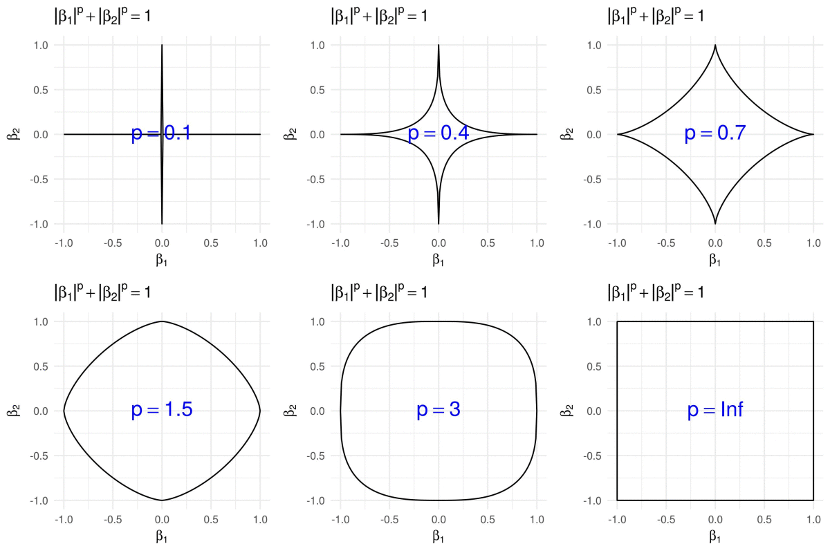

Elastic net penalty in 2D

The elastic net penalty can be written in the form

\[g\subscript{\alpha}(\boldsymbol{\beta}) = \alpha \lVert \boldsymbol{\beta} \rVert\subscript{1} + (1 - \alpha) \lVert \boldsymbol{\beta} \rVert\subscript{2}^{2},\]

for \(\alpha\in(0,1)\). It is quite popular with a variety of regression-based methods (such as the Elastic Net, of course). We obtain the corresponding 2D unit “ball”, by calculating \(\beta\subscript{2}\) from a given \(\beta\subscript{1}\in[-1,1]\) as

\[\beta\subscript{2} = \pm \frac{-\alpha + \sqrt{\alpha^2 - 4 (1 - \alpha) ((1 - \alpha) \beta\subscript{1}^2 + \alpha \beta\subscript{1} - 1)}}{2 - 2 \alpha}.\]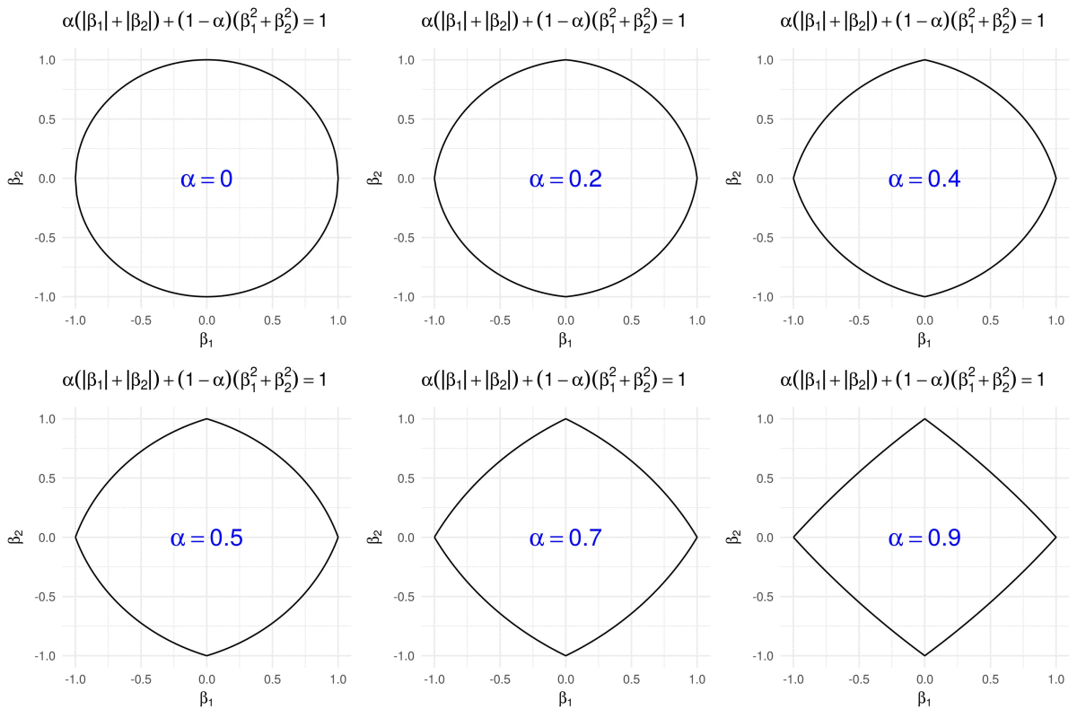

Fused penalty in 2D

The fused penalty can be written in the form

\[g\subscript{\alpha}(\boldsymbol{\beta}) = \alpha \lVert \boldsymbol{\beta} \rVert\subscript{1} + (1 - \alpha) \sum\subscript{i = 2}^m \lvert \beta\subscript{i} - \beta\subscript{i-1} \rvert.\]

It encourages neighboring coefficients \(\beta\subscript{i}\) to have similar values, and is utilized by the fused LASSO (Tibshirani et. al. 2005) and similar methods.

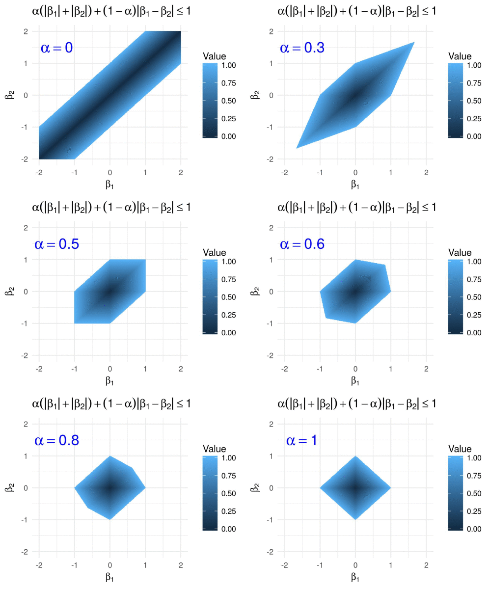
(Here I have simply evaluated the fused penalty function on a grid of points in \([-2,2]^2\), because figuring out equations in parametric form for the above polygons was too painful for my taste… )

Sorted L1 penalty in 2D

The Sorted \(\ell\subscript{1}\) penalty is used in a number of regression-based methods, such as SLOPE (Bogdan et. al. 2015) and OSCAR (Bondell and Reich 2008). It has the form

\[g\subscript{\boldsymbol{\lambda}}(\boldsymbol{\beta}) = \sum\subscript{i = 1}^m \lambda\subscript{i} \lvert \beta \rvert\subscript{(i)},\]

where \(\lvert \beta \rvert\subscript{(1)} \geq \lvert \beta \rvert\subscript{(2)} \geq \ldots \geq \lvert \beta \rvert\subscript{(m)}\) are the absolute values of the entries of \(\boldsymbol{\beta}\) arranged in a decreasing order. In 2D this reduces to

\[g\subscript{\boldsymbol{\lambda}}(\boldsymbol{\beta}) = \lambda\subscript{1} \max\{|\beta\subscript{1}|, |\beta\subscript{2}|\} + \lambda\subscript{2} \min\{|\beta\subscript{1}|, |\beta\subscript{2}|\}.\]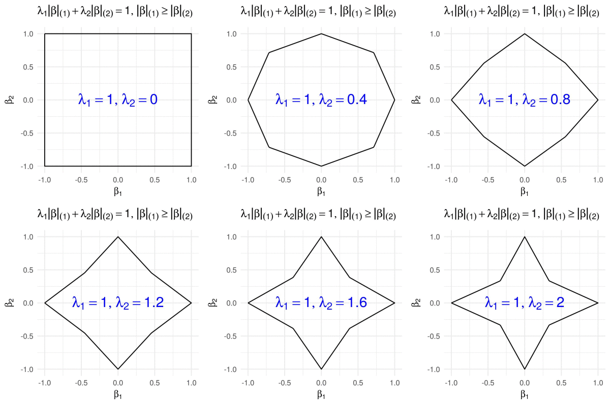

Difference of p-norms

It holds that

\[\lVert \boldsymbol{\beta} \rVert\subscript{1} \geq \lVert \boldsymbol{\beta} \rVert\subscript{2},\]

or more generally, for all \(p\)-norms it holds that

\[(\forall p \leq q) : \lVert \boldsymbol{\beta} \rVert\subscript{p} \geq \lVert \boldsymbol{\beta} \rVert\subscript{q}.\]

Thus, it is meaningful to define a penalty function of the form

\[g\subscript{\alpha}(\boldsymbol{\beta}) = \lVert \boldsymbol{\beta} \rVert\subscript{1} - \alpha \lVert \boldsymbol{\beta} \rVert\subscript{2},\]

for \(\alpha\in[0,1]\), which results in the following.

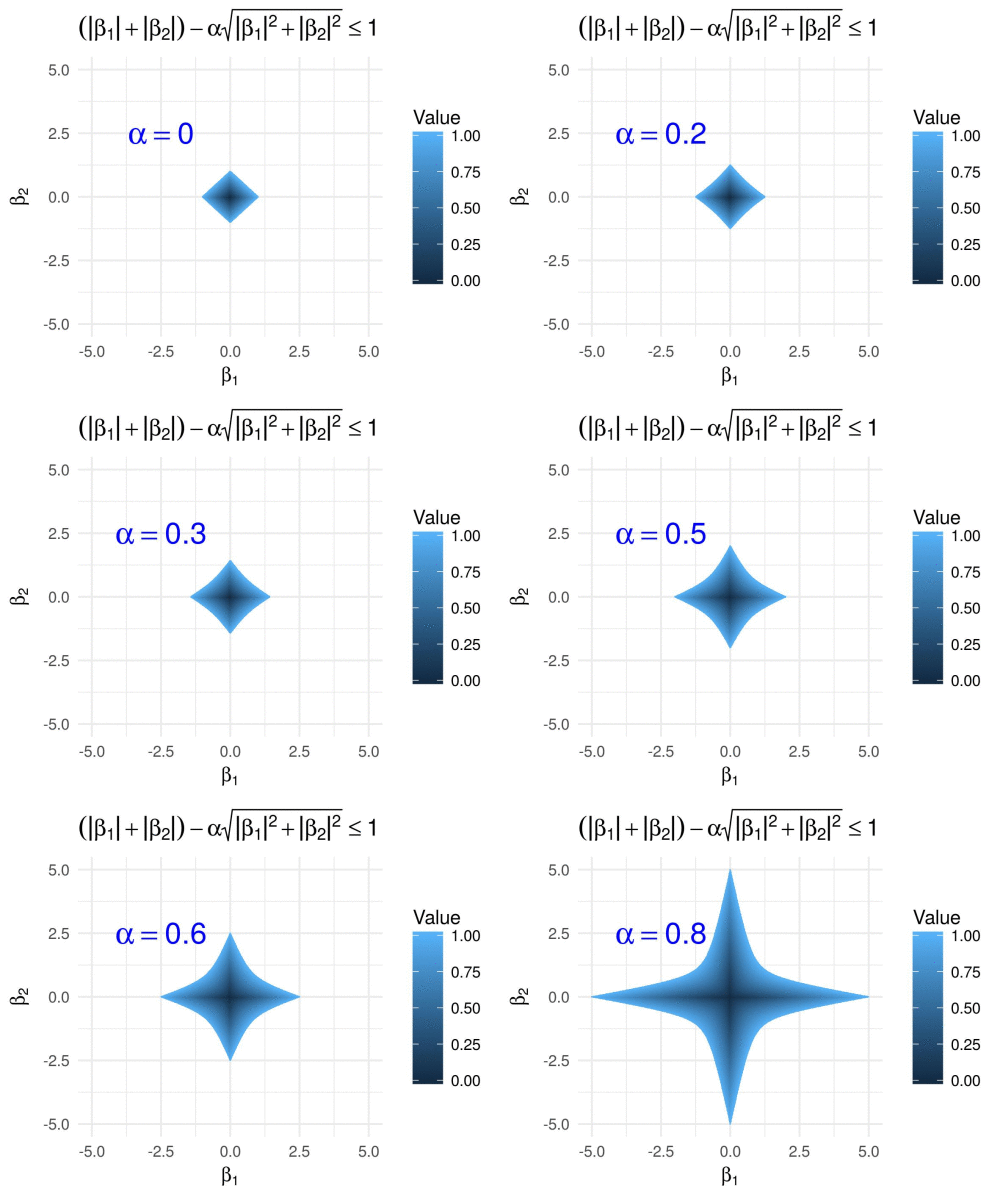
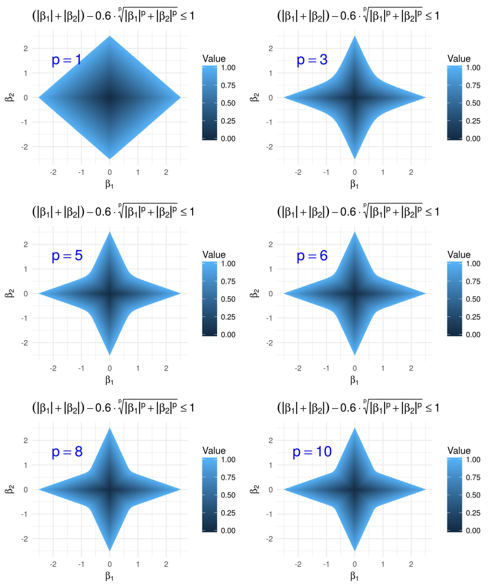
We visualize the same for varying \(p \geq 1\) fixing \(\alpha = 0.6\), i.e., we define

\[g\subscript{\alpha}(\boldsymbol{\beta}) = \lVert \boldsymbol{\beta} \rVert\subscript{1} - 0.6 \lVert \boldsymbol{\beta} \rVert\subscript{p},\]

and we obtain the following GIF.

Hyperbolic tangent penalty in 2D

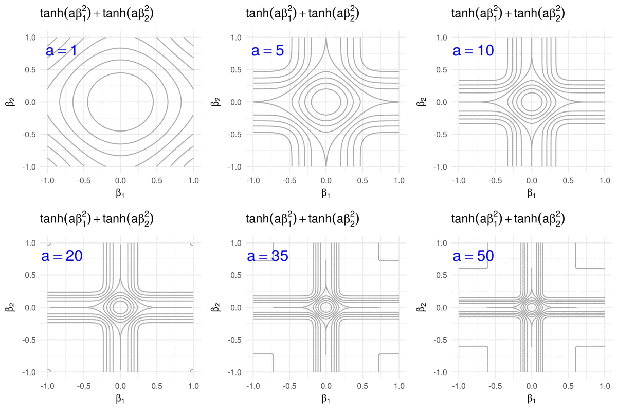
The hyperbolic tangent penalty, which is for example used in the method of variable selection via subtle uprooting (Su, 2015), has the form

\[g\subscript{a}(\boldsymbol{\beta}) = \sum\subscript{i = 1}^p \tanh(a \beta\subscript{i}^2), \quad a>0.\]

Contrary to all of the previously shown penalty functions, for any fixed \(a\) the hyperbolic tangent penalty has round contours (for small values of \(g\subscript{a}\)) as well as contours with sharp corners (for larger values of \(g\subscript{a}\)).

Code

The R code uses the libraries dplyr for data manipulation, ggplot2 for generation of figures, and magick to combine the individual images into a GIF.

Here are the R scripts that can be used to reproduce the above GIFs:

Should I come across other interesting penalty functions that make sense in 2D, then I will add corresponding further visualizations to the same Github repository.

This work is licensed under a Creative Commons Attribution 4.0 International License.